Disclaimer: I am far from an an expert on infectious disease modelling! My knowledge is mostly from university courses on the topic.

My last post explains the background and provides an introduction to the topic of modelling infectious diseases. You might want to read that first to understand this one if you don’t already know the SIR equations. This article is focused on more elaborate variants of the basic SIR model and will enable you to implement and code your own variants and ideas. Another post is concerned with fitting a model to real-world data and includes Covid-19 as a case study.

You can find the notebook with the whole code for this post here.

First, we’ll quickly explore the SIR model from a slightly different - more visual - angle. Afterwards, we derive and implement the following extensions:

• a “Dead” state for individuals that passed away from the disease
• an “Exposed” state for individuals that have contracted the disease but are not yet infectious (this is known as the SEIR-model)
• time-dependent R₀-values that will allow us to model quarantines, lockdowns, …
• resource- and age-dependent fatality rates that will enable us to model overcrowded hospitals, populations with lots of young people, …

Models as State Transitions

As a quick recap, take a look at the variables we defined:

• N: total population
• S(t): number of people susceptible on day t
• I(t): number of people infected on day t
• R(t): number of people recovered on day t
• β: expected amount of people an infected person infects per day
• D: number of days an infected person has and can spread the disease
• γ: the proportion of infected recovering per day (γ = 1/D)
• R₀: the total number of people an infected person infects (R₀ = β / γ)

And here are the basic equations again:

When deriving the equations, we already intuitively thought of them as “directions” that tell us what happens to the population the next day (for example, when 10 people are infected and recovery takes place at the rate 1/5 (that’s gamma), then the number of recovered individuals the next day should increase by 1/5 * 10 = 2). We now solidify this understanding of the equations as “directions” or “transitions” from one compartment S, I or R to another - this will greatly simplify things when we introduce more compartments later on and the equations get messy.

Here’s the notation we need:

Compartments are boxes (the “states”), like this:

Transitions from one compartment to another are represented by arrows, with the following labeling:

The rate describes how long the transition takes, population is the group of individuals that this transition applies to, and probability is the probability of the transition taking place for an individual.

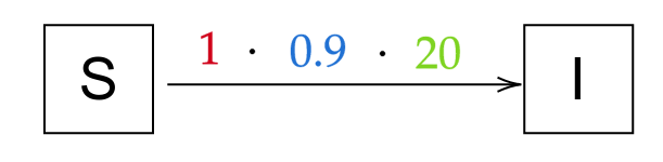
As an example, let’s look at the transition from Susceptibles to Infected in our SIR equations, with beta=2, a total population of 100, 10 infected and 90 susceptible. The rate is 1, as the infections happen immediately; the population the transition applies to is 2 * 10 = 20 individuals, as the 10 infected each infect 2 people; the probability is 90%, as 90/100 people can still be infected. It corresponds to this intuitive notation:

And more generally, now for the whole model (for I → R, the rate is γ and the probability is 1 as everyone recovers):

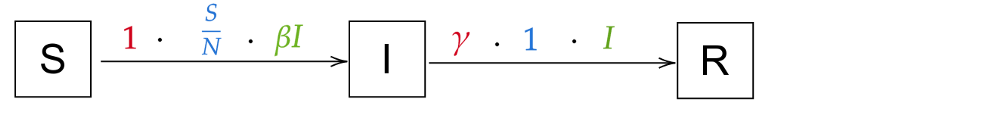
As you can see, arrows pointing towards a compartment get added in the equation; arrows pointing away from a compartment get subtracted. That’s not too bad, is it? Take a moment to really understand the new notation and see how it is just another way of writing the equations.

Right, we now understand the SIR model and can code it in python, but is it already useful? Can it tell us anything about real-world infectious diseases? The answer is no. In its current state, the model is more of a toy than a useful tool. Let’s change that!

Introducing new Compartments

Deriving the Exposed-Compartment

Many infectious diseases have an incubation period before being infectious during which the host cannot yet spread the disease. We’ll call such individuals - and the whole compartment - Exposed.

Intuitively, we’ll have transitions of the form S → E → I → R: Susceptible people can contract the virus and thus become exposed, then infected, then recovered. The new transition S → E will have the same arrow as the current S → I transition, as the probability is the same (all susceptibles can be exposed), the rate is the same (“exposition” happens immediately) and the population is the same (the infectious individuals can spread the disease and each exposes β new individuals per day). There’s also no reason for the transition from I to R to change. The only new transition is the one from E to I: the probability is 1 (everyone that’s exposed becomes infected), the population is E (all exposed will become infected), and the rate gets a new variable, δ (delta). We arrive at these transitions:

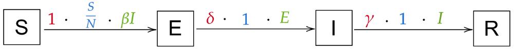
From these transitions, we can immediately derive these equations (again, compare the state transitions and the equations until it makes sense to you):

Programming the Exposed-Compartment

This should not be too hard, we just have to change a few lines of code from the last article (again, the full code is here to read along, I’m just showcasing the important bits here). We’ll model a highly infectious (R₀ =5.0) disease in a population of 1 million, with an incubation period of 5 days and a recovery taking 7 days.

def deriv(y, t, N, beta, gamma, delta):
    S, E, I, R = y
    dSdt = -beta * S * I / N
    dEdt = beta * S * I / N - delta * E
    dIdt = delta * E - gamma * I
    dRdt = gamma * I
    return dSdt, dEdt, dIdt, dRdt

N = 1000
beta = 1.0  # infected person infects 1 other person per day
D = 4.0 # infections lasts four days
gamma = 1.0 / D
delta = 1.0 / 3.0  # incubation period of three days

S0, E0, I0, R0 = 999, 1, 0, 0  # initial conditions: one exposed, rest susceptible

We calculate S, E, I, and R over time:

t = np.linspace(0, 100, 100) # Grid of time points (in days)
y0 = S0, E0, I0, R0 # Initial conditions vector

# Integrate the SIR equations over the time grid, t.
ret = odeint(deriv, y0, t, args=(N, beta, gamma, delta))
S, E, I, R = ret.T

And we get this:

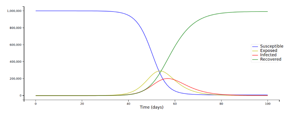
We are now able to model real diseases a little more realistically, though one compartment is definitely still missing; we’ll add it now:

Deriving the Dead-Compartment

For very deadly diseases, this compartment is very important. For some other situations, you might want to add completely different compartments and dynamics (such as births and non-disease-related deaths when studying a disease over a long time); these models can get as complex as you want!

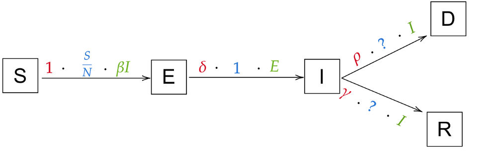
Here are our current transitions once more:

Let’s think about how we can take our current transitions and add a Dead state. When can people die from the disease? Only while they are infected! That means that we’ll have to add a transition I → D. Of course, people don’t die immediately; We define a new variable ρ (rho) for the rate at which people die (e.g. when it takes 6 days to die, ρ will be 1/6). There’s no reason for the rate of recovery, γ, to change. So our new model will look similar to this:

The only thing that’s missing are the probabilities of going from infected to recovered and from infected to dead. That’ll be one more variable (the last one for now!), the death rate α. For example, if α=5%, ρ = 1 and γ = 1 (so people die or recover in 1 day, that makes for an easier example) and 100 people are infected, then 5% ⋅ 100 = 5 people will die. That leaves 95% ⋅ 100 = 95 people recovering. So all in all, the probability for I → D is α and thus the probability for I → R is 1-α. We finally arrive at this model:

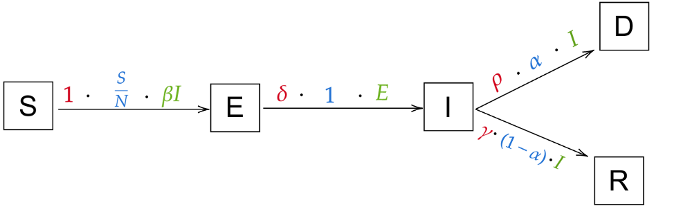
Which naturally translates to these equations:

Programming the Dead-Compartment

We only need to make some slight changes to the code (and we’ll set α to 20% and ρ to 1/9)…

def deriv(y, t, N, beta, gamma, delta, alpha, rho):
    S, E, I, R, D = y
    dSdt = -beta * S * I / N
    dEdt = beta * S * I / N - delta * E
    dIdt = delta * E - (1 - alpha) * gamma * I - alpha * rho * I
    dRdt = (1 - alpha) * gamma * I
    dDdt = alpha * rho * I
    return dSdt, dEdt, dIdt, dRdt, dDdt


N = 1_000_000
D = 4.0 # infections lasts four days
gamma = 1.0 / D
delta = 1.0 / 5.0  # incubation period of five days
R_0 = 5.0
beta = R_0 * gamma  # R_0 = beta / gamma, so beta = R_0 * gamma
alpha = 0.2  # 10% death rate
rho = 1/9  # 9 days from infection until death
S0, E0, I0, R0, D0 = N-1, 1, 0, 0, 0  # initial conditions: one exposed


t = np.linspace(0, 100, 100) # Grid of time points (in days)
y0 = S0, E0, I0, R0, D0 # Initial conditions vector

# Integrate the SIR equations over the time grid, t.
ret = odeint(deriv, y0, t, args=(N, beta, gamma, delta, alpha, rho))
S, E, I, R, D = ret.T

… and we arrive at this:

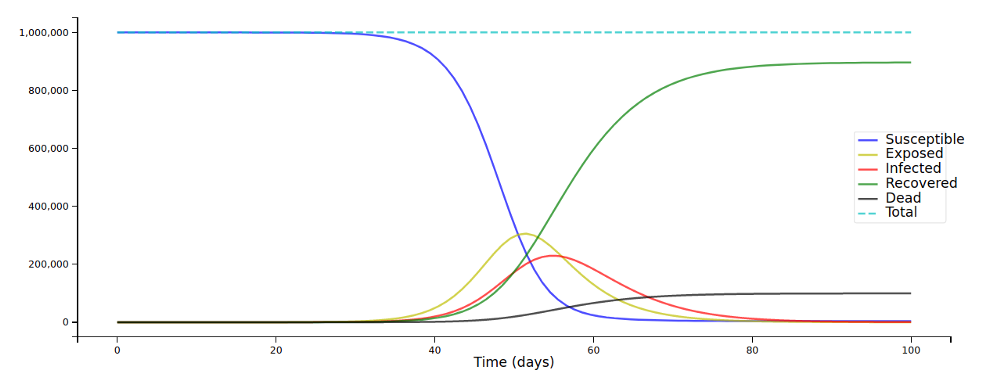
Note that I added a “total” that adds up S, E, I, R, and D for every time step as a “sanity check”: The compartments always have to sum up to N; this can give you a hint as to whether your equations are correct.

You should now know how you can add a new compartment to the model: Think about what transitions need to be added and changed; think about the probabilities, populations and rates of these new transitions; draw the diagram; and finally write down the equations. The coding is definitively not the hard part for these models!

For example, you might want to add a “ICU” compartment for infected individuals that need to go to an ICU (we’ll do that in the next article). Think about from which compartment people can go to the ICU, where they can go after the ICU, etc.

Time-Dependent Variables

Here’s an updated list of the variables we currently use:

• N: total population
• S(t): number of people susceptible on day t
• E(t): number of people exposed on day t
• I(t): number of people infected on day t
• R(t): number of people recovered on day t
• D(t): number of people dead on day t
• β: expected amount of people an infected person infects per day
• D: number of days an infected person has and can spread the disease
• γ: the proportion of infected recovering per day (γ = 1/D)
• R₀: the total number of people an infected person infects (R₀ = β / γ)
• δ: length of incubation period
• α: fatality rate
• ρ: rate at which people die (= 1/days from infected until death)

As you can see, only the compartments change over time (they are not constant). Of course, this is highly unrealistic! As an example, why should the R₀-value be constant? Surely, nationwide lockdowns reduce the number of people an infected person infects, that’s what they’re all about! Naturally, to get closer to modelling real-world developments, we have to make our variables change over time.

Time-Dependent R₀

First, we implement a simple change: on day L, a strict “lockdown” is enforced, pushing R₀ to 0.9. In the equations, we use β and not R₀, but we know that R₀ = β / γ, so β = R₀ ⋅ γ. That means that we define a function

def R_0(t):
    return 5.0 if t < L else 0.9

and another function for beta that calls this function:

def beta(t):
    return R_0(t) * gamma

Right, seems easy enough! We just change the code accordingly:

def deriv(y, t, N, beta, gamma, delta, alpha, rho):
    S, E, I, R, D = y
    dSdt = -beta(t) * S * I / N
    dEdt = beta(t) * S * I / N - delta * E
    dIdt = delta * E - (1 - alpha) * gamma * I - alpha * rho * I
    dRdt = (1 - alpha) * gamma * I
    dDdt = alpha * rho * I
    return dSdt, dEdt, dIdt, dRdt, dDdt


L = 100

N = 1_000_000
D = 4.0 # infections lasts four days
gamma = 1.0 / D
delta = 1.0 / 5.0  # incubation period of five days
def R_0(t):
    return 5.0 if t < L else 0.9
def beta(t):
    return R_0(t) * gamma

alpha = 0.2  # 20% death rate
rho = 1/9  # 9 days from infection until death
S0, E0, I0, R0, D0 = N-1, 1, 0, 0, 0  # initial conditions: one exposed


t = np.linspace(0, 100, 100) # Grid of time points (in days)
y0 = S0, E0, I0, R0, D0 # Initial conditions vector

# Integrate the SIR equations over the time grid, t.
ret = odeint(deriv, y0, t, args=(N, beta, gamma, delta, alpha, rho))
S, E, I, R, D = ret.T

plotseird(t, S, E, I, R, D)

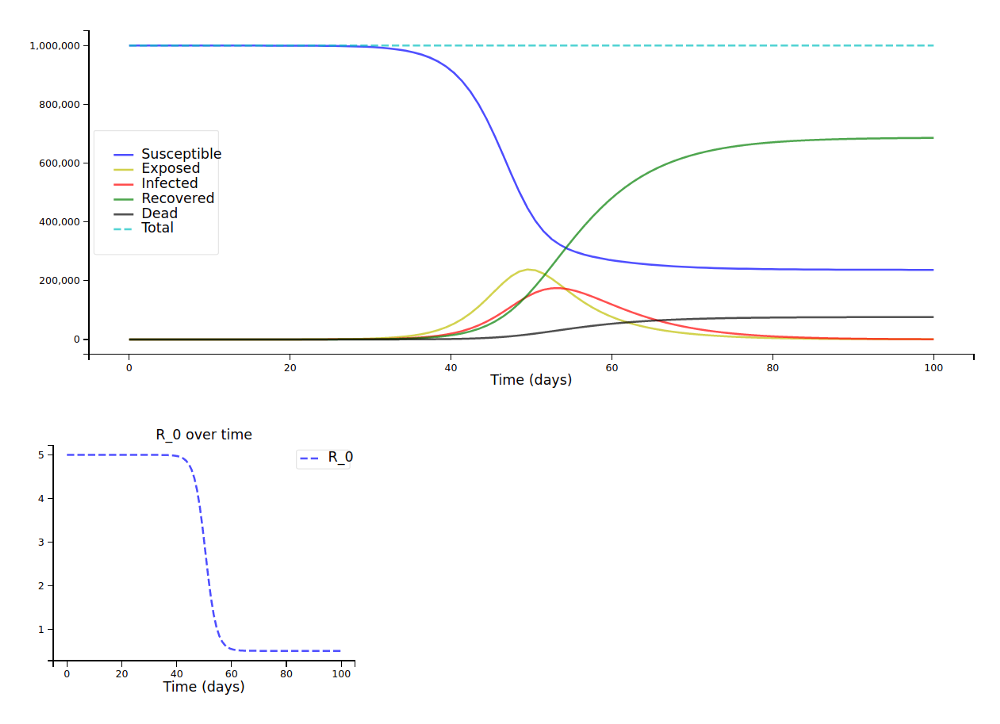
Let’s plot this for some different values of L:

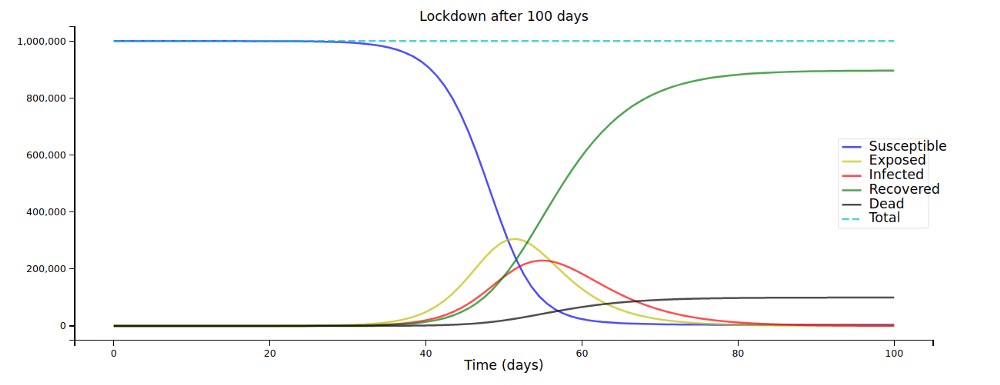
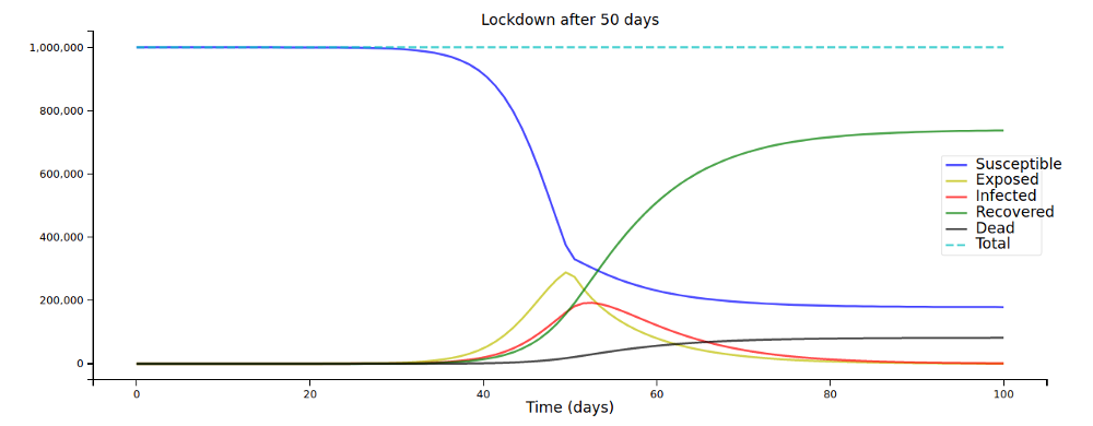
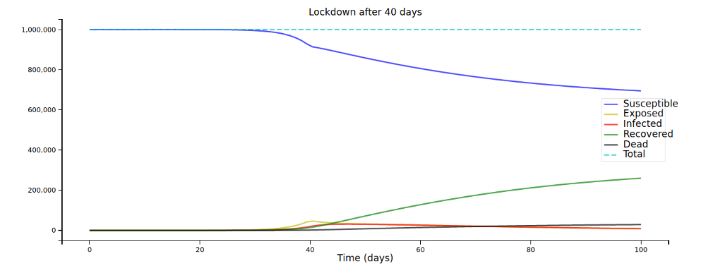
A few days can make a huge difference in the overall spread of the disease!

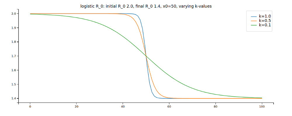
In reality, R₀ probably never “jumps” from one value to another. Rather, it (more or less quickly) continuously changes (and might go up and down several times, e.g. if social distancing measures are loosened and then tightened again). You can choose any function you want for R₀, I just want to present one common choice to model the initial impact of social distancing: a logistic function.

The function (adopted for our purposes) looks like this:

And here’s what the parameters actually do:

• R_0_start and R_0_end are the values of R_0 on the first and the last day
• x_0 is the x-value of the inflection point (i.e. the date of the steepest decline in R_0, this could be thought of as the main “lockdown” date)
• k lets us vary how quickly R_0 declines

These plots might help you understand the parameters:

Again, changing the code accordingly:

def deriv(y, t, N, beta, gamma, delta, alpha, rho):
    S, E, I, R, D = y
    dSdt = -beta(t) * S * I / N
    dEdt = beta(t) * S * I / N - delta * E
    dIdt = delta * E - (1 - alpha) * gamma * I - alpha * rho * I
    dRdt = (1 - alpha) * gamma * I
    dDdt = alpha * rho * I
    return dSdt, dEdt, dIdt, dRdt, dDdt


N = 1_000_000
D = 4.0 # infections lasts four days
gamma = 1.0 / D
delta = 1.0 / 5.0  # incubation period of five days

R_0_start, k, x0, R_0_end = 5.0, 0.5, 50, 0.5

def logistic_R_0(t):
    return (R_0_start-R_0_end) / (1 + np.exp(-k*(-t+x0))) + R_0_end

def beta(t):
    return logistic_R_0(t) * gamma

alpha = 0.2  # 20% death rate
rho = 1/9  # 9 days from infection until death
S0, E0, I0, R0, D0 = N-1, 1, 0, 0, 0  # initial conditions: one exposed


t = np.linspace(0, 100, 100) # Grid of time points (in days)
y0 = S0, E0, I0, R0, D0 # Initial conditions vector

# Integrate the SIR equations over the time grid, t.
ret = odeint(deriv, y0, t, args=(N, beta, gamma, delta, alpha, rho))
S, E, I, R, D = ret.T
R0_over_time = [logistic_R_0(i) for i in range(len(t))]  # to plot R_0 over time: get function values

We let R₀ decline quickly from 5.0 to 0.5 around day 50 and can now really see the curves flattening after day 50:

Resource- and Age-Dependent Fatality Rates

Similarly to R₀, the fatality rate α is probably not constant for most real diseases. It might depend on a variety of things; We’ll focus on dependency on resources and age.

First, let’s look at resource dependency. We want the fatality rate to be higher when more people are infected. Think about how this could be put into a function: we probably need a “base” or “optimal” fatality rate for the case that only few people are infected (and thus receive optimal treatment) and some factor that takes into account what proportion of the population is currently infected. This is one example of a function that implements these ideas:

Here, s is some arbitrary but fixed (that means we choose it freely once for a model and then it stays constant over time) scaling factor that controls how big of an influence the proportion of infected should have; α_OPT is the optimal fatality rate. For example, if s=1 and half the population is infected on one day, then s ⋅ I(t) / N = 1/2, so the fatality rate α(t) on that day is 50% + α_OPT. Or maybe most people barely have any symptoms and thus many people being infected does not clog the hospitals. Then a scaling factor of 0.1 might be appropriate (in the same scenario, the fatality rate would only be 5% + α_OPT).

More elaborate models might make the fatality rate depend on the number of ICU beds or ventilators available, etc. We’ll do that in the next article when modelling Coronavirus.

Age dependency is a little more difficult. To fully implement it, we’d have to include separate compartments for every age group (e.g. an Infected-compartment for people aged 0–9, another one for people aged 10–19, …). That’s doable with a simple for-loop in python, but the equations get a little messy. A simpler approach that still is able to produce good results is the following:

We need 2 things for the simpler approach: Fatality rates by age group and proportion of the total population that is in that age group. For example, we might have the following fatality rates and number of individuals by age group (in Python dictionaries):

alpha_by_agegroup = {
    "0-29": 0.01, "30-59": 0.05, "60-89": 0.20, "89+": 0.30
}
proportion_of_agegroup = {
    "0-29": 0.1, "30-59": 0.3, "60-89": 0.4, "89+": 0.2
}

(This would be an extremely old population with 40% being in the 60–89 range and 20% being in the 89+ range). Now we calculate the overall average fatality rate by adding up the age group fatality rate multiplied with the proportion of the population in that age group:

α = 0.01 ⋅ 0.1 + 0.05 ⋅ 0.3 + 0.2 ⋅ 0.4 + 0.3 ⋅ 0.2 = 15.6%. Or in code:

alpha = sum(alpha_by_agegroup[agegroup] * proportion_of_agegroup[agegroup]
            for agegroup in alpha_by_agegroup.keys())

A rather young population with the following proportions …

proportion_of_agegroup = {
    "0-29": 0.4, "30-59": 0.4, "60-89": 0.1, "89+": 0.1
}

… would only have an average fatality rate of 7.4%!

If we want to use both our formulas for resource- and age-dependency, we could use the resource-formula we just used to calculate α_OPT and use that in our resource-dependent formula from above.

There are certainly more elaborate ways to implement fatality rates over time. For example, we’re not taking into account that only critical cases needing intensive care fill up the hospitals and might increase fatality rates; or that deaths change the population structure that we used to calculate the fatality rate in the first place; or that the impact of infected on fatality rates should take place several days later as people don’t usually die immediately, which would result in a Delay Differential Equation, and that’s a bit more annoying to deal with in Python! Again, get as creative as you want!

Implementing Resource- and Age-Dependent Fatality Rates

This is rather straightforward, we don’t even have to change our main equations (we define alpha inside the equations as we need access to the current value I(t)).

def deriv(y, t, N, beta, gamma, delta, alpha_opt, rho):
    S, E, I, R, D = y
    def alpha(t):
        return s * I/N + alpha_opt

    dSdt = -beta(t) * S * I / N
    dEdt = beta(t) * S * I / N - delta * E
    dIdt = delta * E - (1 - alpha(t)) * gamma * I - alpha(t) * rho * I
    dRdt = (1 - alpha(t)) * gamma * I
    dDdt = alpha(t) * rho * I
    return dSdt, dEdt, dIdt, dRdt, dDdt


N = 1_000_000
D = 4.0 # infections lasts four days
gamma = 1.0 / D
delta = 1.0 / 5.0  # incubation period of five days

R_0_start, k, x0, R_0_end = 5.0, 0.5, 50, 0.5

def logistic_R_0(t):
    return (R_0_start-R_0_end) / (1 + np.exp(-k*(-t+x0))) + R_0_end

def beta(t):
    return logistic_R_0(t) * gamma

alpha_by_agegroup = {"0-29": 0.01, "30-59": 0.05, "60-89": 0.2, "89+": 0.3}
proportion_of_agegroup = {"0-29": 0.1, "30-59": 0.3, "60-89": 0.4, "89+": 0.2}
s = 1.0
alpha_opt = sum(alpha_by_agegroup[i] * proportion_of_agegroup[i] for i in list(alpha_by_agegroup.keys()))

rho = 1/9  # 9 days from infection until death
S0, E0, I0, R0, D0 = N-1, 1, 0, 0, 0  # initial conditions: one exposed


t = np.linspace(0, 100, 100) # Grid of time points (in days)
y0 = S0, E0, I0, R0, D0 # Initial conditions vector

# Integrate the SIR equations over the time grid, t.
ret = odeint(deriv, y0, t, args=(N, beta, gamma, delta, alpha_opt, rho))
S, E, I, R, D = ret.T
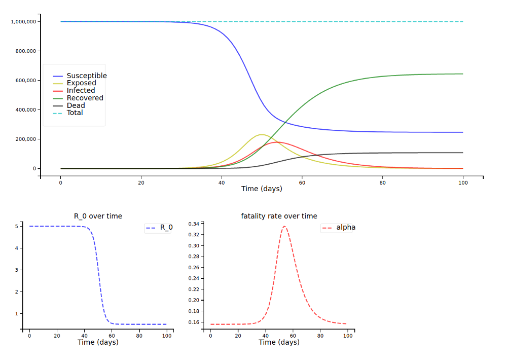
R0_over_time = [logistic_R_0(i) for i in range(len(t))]  # to plot R_0 over time: get function values
Alpha_over_time = [s * I[i]/N + alpha_opt for i in range(len(t))]  # to plot alpha over time


plotseird(t, S, E, I, R, D, R0=R0_over_time, Alpha=Alpha_over_time)

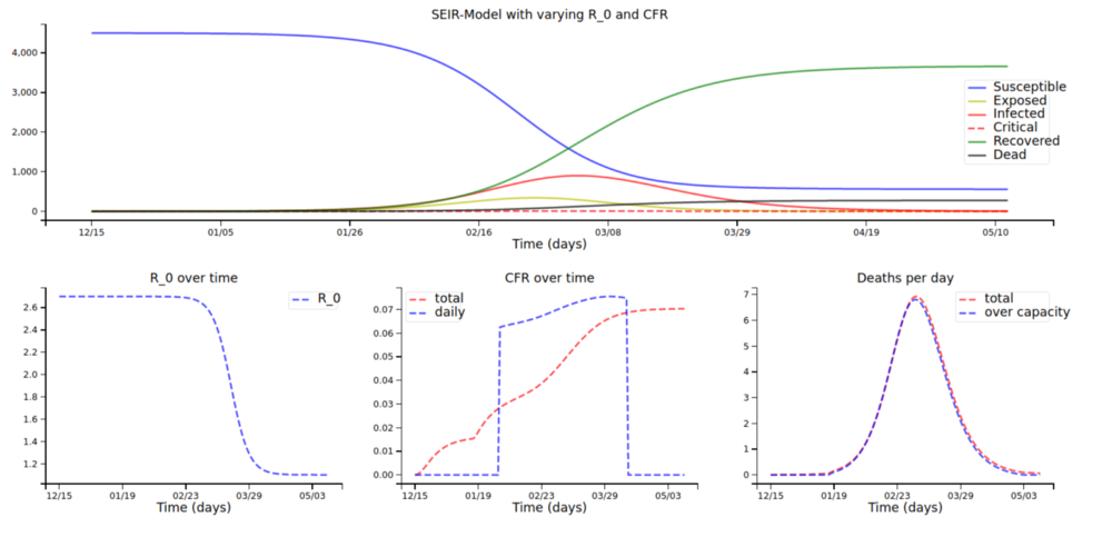
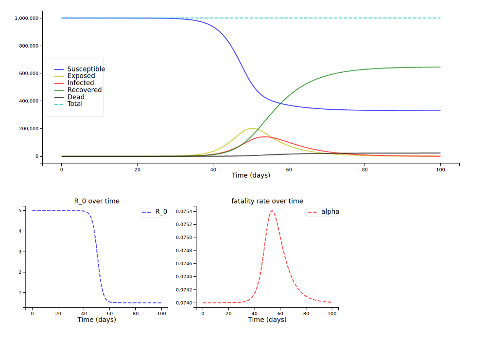
With the fatality rates by age group and the older population from above (and a scaling factor s of 1, so many people being infected has a high impact on fatality rates), we arrive at this plot:

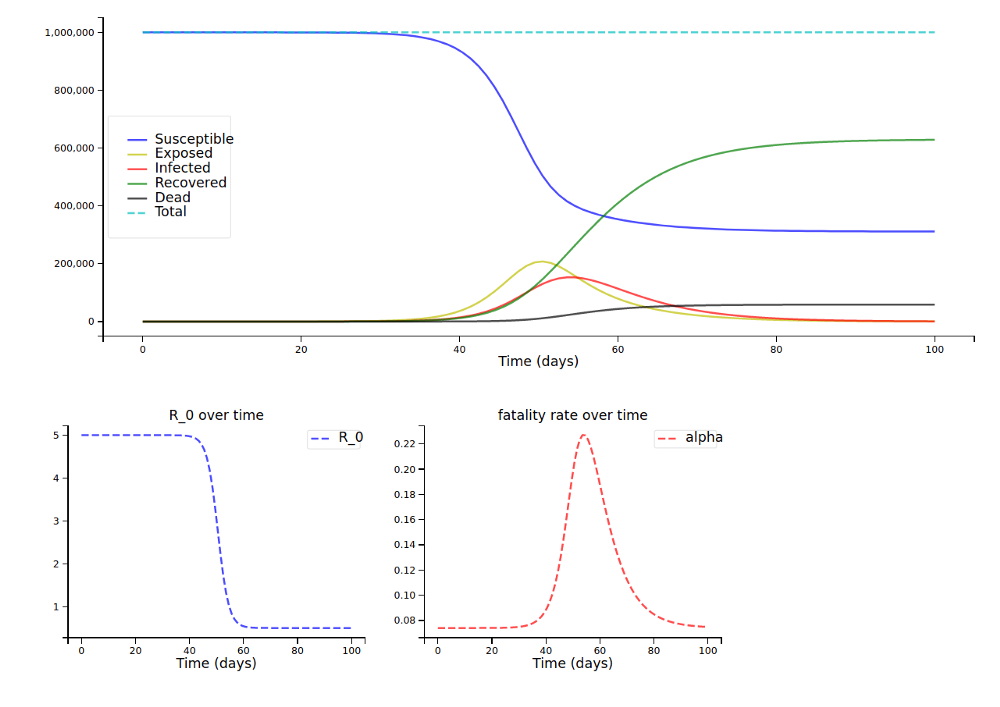
For the younger population (around 80k instead of 150k deaths):

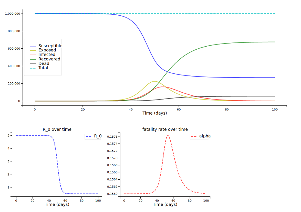
And now with a scaling factor of only 0.01:

For the older population (note how the fatality rate only rises very slightly over time) …

… and the younger population:

Recap

That’s all! You should now be able to add your own compartments (maybe a compartment for individuals that can get infected again, or a compartment for a special risk group such as diabetics), first graphically through the state transition notation, then formally through the equations, and finally programmatically in Python! Also, you saw some examples of implementing time-dependent variables, making the models much more versatile.

All this should allow you to design SIR models that come quite close to the real world. Of course, many scientists are working on these models currently (this link can help you find some current articles - be warned, they can get quite complex, but it’s nonetheless a great way to get insights into the current state of the field). In the next post, we’ll look at designing and fitting models to real-world data, with Coronavirus as a case-study.