Infectious Disease Modelling I: Understanding the Models That Are Used to Model Coronavirus
Disclaimer: I am far from an an expert on infectious disease modelling! My knowledge is mostly from university courses on the topic.
In the past few weeks, lots of data scientists, hobbyists, and enthusiasts have begun to read about infectious disease modelling (me included!). Many of them have jumped right into modelling and fitting their models to covid case numbers without looking at the background and theory behind the models. Although consisting of seemingly daunting mathematics, the most widely used models are actually not that difficult to understand.
This post explains the background and provides an introduction to the topic of modelling infectious diseases. The SIR model equations are derived and explained from scratch with simple examples. At the end, a simple SIR model is coded in Python. My next post is focused on more elaborate variants of the basic SIR model and will enable readers to implement and visualize their own variants and ideas. Another post is concerned with fitting a model to real-world data and includes covid as a case study.
You can find the notebook with the whole code for this post here.
Some Background
This post is not meant to quickly show you some plots with lots of colorful curves that are supposed to convince you that my model can perfectly predict covid cases; Rather, I’ll try to explain all the background necessary for you to understand these models, form your own opinion of these models and implement your own ideas. You only need high school level calculus to follow the explanations; You’ll need some understanding of Python to follow the programming parts.
So, with that in mind:
We want to model infectious diseases. These diseases can spread from one member of a population to another; we try to gain insights into how quickly they spread, what proportion of a population they infect, what proportion dies, etc. One of the easiest ways to model them (and the way we’re focusing on here) is with a compartmental model. A compartmental model separates the population into several compartments, for example:
- Susceptible (can still be infected, ‘healthy’)
- Infected
- Recovered
That is, we might have a population of N=1000 (for example 1000 people) and we know that 400 people are infected at time t (for example t=7 days after outbreak of the disease). This is denoted by S(7) = 400. The SIR-Model allows us to, only by inputting some initial parameters, get all values S(t), I(t), R(t) for all days t. Let’s look at the necessary variables with an easy example:
Assume we have a new disease, disease X. For this disease, the probability of an infected person to infect a healthy person is 20%. The average number of people a person is in contact with per day is 5. So, per day, an infected individual meets 5 people and infects each with 20% probability. Thus, we expect this individual to infect 1 person (20% ⋅ 5 = 1) per day. This is β (“beta”), the expected amount of people an infected person infects per day.
Now one can see that the number of days that an infected person has and can spread the disease is extremely important. We’ll call this number D. If D=7, an infected person walks around for seven days spreading the disease, and infects 1 person per day (because β=1). So we expect an infected person to infect 1⋅7 (1 per day times 7 days) = 7 other people. This is the basic reproduction number R₀, the total number of people an infected person infects. We just used an intuitive formula: R₀ = β ⋅ D.
We actually don’t need anything else, just one small notation: γ (“gamma”) will be 1/D, so if you think of D as the number of days an infected person has the disease, you can think of γ as the rate of recovery, or the proportion of infected recovering per day. For example, if currently 30 people are infected and D=3 (so they’re infected for three days), then per day, 1/3 (so 10) of them will recover, so γ=1/3. With γ = 1/D, so D = 1/γ , and R₀ = β ⋅ D, it follows that R₀ = β / γ.
Here you can see the most important variables and their definitions again:
- N: total population
- S(t): number of people susceptible on day t
- I(t): number of people infected on day t
- R(t): number of people recovered on day t
- β: expected amount of people an infected person infects per day
- D: number of days an infected person has and can spread the disease
- γ: the proportion of infected recovering per day (γ = 1/D)
- R₀: the total number of people an infected person infects (R₀ = β / γ)
Deriving the Formulas
We now want to get the number of infected, susceptible, and recovered people for all days, just from β, γ and N. Now, it is difficult to obtain a direct formula for S(t), I(t) and R(t). However, it is quite simple to describe the change per day of S, I, and R, that is, how the number of susceptible/infected/recovered changes depending on the current numbers. Again, we’ll derive the formulas by example:
Assume we are now on day t after outbreak of disease X. Still, the expected amount of people an infected person infects per day is 1 (so β=1) and the number of days that an infected person has and can spread the disease is 7 (so γ=1/7 and D=7).
Let’s say that on day t, 60 people are infected (so I(t)=60), the total population is 100 (so N=100), and 30 people are still susceptible (so S(t)=30 and R(t)=100–60–30=10). Now, how do S(t) and I(t) and R(t) change to the next day?
We have 60 infected people. Each of them infects 1 person per day (that’s β). However, only 30/100 =30% of people they meet are still susceptible and can be infected (that’s S(t) / N). So, they infect 60 ⋅ 1 ⋅ 30/100 = 18 people (again, think about it until it really makes sense: 60 infected that infect on average 1 person per day, but only 30 of 100 people can still be infected, so they do not infect 60⋅1 people, but only 60⋅1⋅30/100 = 18 people). So, 18 people of the susceptibles get infected, so S(t) changes by minus 18. Plugging in the variables, we just derived the first formula:
Change of S(t) to the next day = - β ⋅ I(t) ⋅ S(t) / N.
If you’re familiar with calculus, you know we have a term for describing the change of a function: the derivative S’(t) or dS/dt. (After we have derived and understood all the derivatives S’(t), I’(t) and R’(t), we can calculate the values of S(t), I(t) and R(t) for each day.)
So: S’(t) =- β ⋅ I(t) ⋅ S(t) / N
Now, how does the amount of infected change? That’s easy: There are some new people infected, we just saw that. Exactly the amount of people that “leave” S(t) “arrive” at I(t). So, we have 18 new infected and we already know that the formula will be similar to this: I’(t) = + β ⋅ I(t) ⋅ S(t) / N (of course, we can omit the plus, it’s just to show you that we gain the exact amount that S(t) loses, so we just change the sign). There’s just one thing missing: some people recover. Remember, we have γ for that, it’s the proportion of infected recovering per day, that’s just what we need!
We have 60 infected and γ=1/3, so one third of the 60 recovers. That’s 1/3 ⋅ 60 = 20. Finally, we obtain the formula:
I’(t) = β ⋅ I(t) ⋅ S(t) / N -γ ⋅ I(t)
Again, think about this for a minute; The first part is the newly infected from the susceptibles. The second part is the recoveries.
Finally, we get to the last formula, the change in recoveries. That’s easy: the newly recovered are exactly the 20 we just calculated; there are no people leaving the “recovered”-compartment. Once recovered, they stay immune:
R’(t) = γ ⋅ I(t)
Great, we have now derived (and understood) all the formulas we need! Here they are again with a more common notation for the derivative:

Such equations are called ordinary differential equations (ODEs) (you won’t need any knowledge about them to follow this post).
We can now describe the change in the number of people susceptible, infected, and recovered. From these formulas, luckily, we can calculate the numbers we’re really interested in: S(t), I(t) and R(t), the number of people susceptible, infected, and recovered for each day t. Even better, we do not have to do one bit ourselves, Python provides many tools for solving ODEs!
Implementing the Model in Python
N = 1000
beta = 1.0  # infected person infects 1 other person per day
D = 4.0 # infections lasts four days
gamma = 1.0 / D

S0, I0, R0 = 999, 1, 0  # initial conditions: one infected, rest susceptible
We now implement exactly the formulas we derived above:
def deriv(y, t, N, beta, gamma):
    S, I, R = y
    dSdt = -beta * S * I / N
    dIdt = beta * S * I / N - gamma * I
    dRdt = gamma * I
    return dSdt, dIdt, dRdt
Now this is where the magic happens: we get our values S(t), I(t) and R(t) from the function odeint that takes the formulas we defined above, the initial conditions, and our variables N, β and γ and calculates S, I, and R for 50 days.
t = np.linspace(0, 50, 50) # Grid of time points (in days)
y0 = S0, I0, R0 # Initial conditions vector

# Integrate the SIR equations over the time grid, t.
ret = odeint(deriv, y0, t, args=(N, beta, gamma))
S, I, R = ret.T
Now we just plot the result and arrive at this:
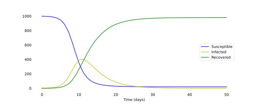
As you can see, it only takes around 30 days for almost a whole population of 1000 people to get infected. Of course, the disease modeled here has a very high R₀ value of 4.0 (recall that R₀ = β ⋅ D = 1.0 ⋅ 4.0). Just changing the number of people an infected person infects per day β to 0.5 results in a completely different scenario:
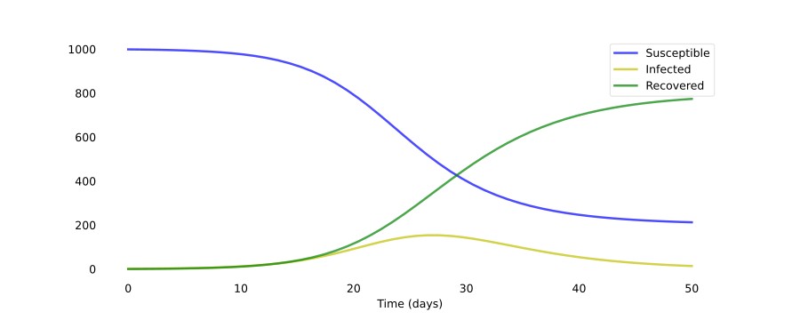
As you can see, these systems of ODEs are extremely sensitive to the initial parameters. That’s also why it’s so hard to correctly model an emerging outbreak of a new disease: we just do not know what the parameters are, and even slight changes result in widely different outcomes.